Identifying True Topics • alto

This vignette applies topic alignment to data generated from a true LDA model. This corresponds to the first simulation in the manuscript accompanying this package. The arguments to this vignette (which can be modified in the original rmarkdown’s YAML) are,

K: The true number of topics underlying the simulated data. In the manuscript, \(K = 5\).
N: The number of samples (i.e., documents) to simulate. In the manuscript, this is set to 250.
V: The number of dimensions (i.e. vocabulary size) per sample. In the manuscript, this is set to 1000.
id: A descriptive ID to associate with any saved results.
method: The alignment strategy to pass to align_topics.
n_models: The total number of models to fit to the simulated data. In the manuscript, this is set to 10.
out_dir: If results are saved, where should they be saved to?
save: Should any results be saved?

The packages used in this vignette are given below. Note that we also load simulation functions from an external github repository (not this package). This provides the simulate_lda function used to generate the data for this example.

library(MCMCpack)
#> Loading required package: coda
#> Loading required package: MASS
#> ##
#> ## Markov Chain Monte Carlo Package (MCMCpack)
#> ## Copyright (C) 2003-2023 Andrew D. Martin, Kevin M. Quinn, and Jong Hee Park
#> ##
#> ## Support provided by the U.S. National Science Foundation
#> ## (Grants SES-0350646 and SES-0350613)
#> ##
library(alto)
#> 
#> Attaching package: 'alto'
#> The following object is masked from 'package:stats':
#> 
#>     weights
library(tidyverse)
#> ── Attaching core tidyverse packages ──────────────────────── tidyverse 2.0.0 ──
#> ✔ dplyr     1.1.0     ✔ readr     2.1.4
#> ✔ forcats   1.0.0     ✔ stringr   1.5.0
#> ✔ ggplot2   3.4.1     ✔ tibble    3.1.8
#> ✔ lubridate 1.9.2     ✔ tidyr     1.3.0
#> ✔ purrr     1.0.1
#> ── Conflicts ────────────────────────────────────────── tidyverse_conflicts() ──
#> ✖ dplyr::filter() masks stats::filter()
#> ✖ dplyr::lag()    masks stats::lag()
#> ✖ dplyr::select() masks MASS::select()
#> ℹ Use the 
source("https://raw.githubusercontent.com/krisrs1128/topic_align/main/simulations/simulation_functions.R")
my_theme()
#> Warning: The `size` argument of `element_rect()` is deprecated as of ggplot2 3.4.0.
#> ℹ Please use the `linewidth` argument instead.

The block below simulates data x according to an LDA models with parameters specified above. The topics are relatively sparse, with \(\lambda_{\beta} = 0.1\) and \(\lambda_{\gamma} = 0.5\). Each sample has 10,000 counts.

attach(params)
lambdas <- list(beta = 0.1, gamma = .5, count = 1e4)
betas <- rdirichlet(K, rep(lambdas$beta, V))
gammas <- rdirichlet(N, rep(lambdas$gamma, K))
x <- simulate_lda(betas, gammas, lambda = lambdas$count)

Next, we run the LDA models and compute the alignment.

lda_params <- map(1:n_models, ~ list(k = .))
names(lda_params) <- str_c("K", 1:n_models)
alignment <- x %>%
  run_lda_models(lda_params, reset = TRUE, dir = "./fits/lda_", seed = as.integer(id)) %>%
  align_topics(method = method)
#> Using default value 'VEM' for 'method' LDA parameter.
#> Using default value 'VEM' for 'method' LDA parameter.
#> Using default value 'VEM' for 'method' LDA parameter.
#> Using default value 'VEM' for 'method' LDA parameter.
#> Using default value 'VEM' for 'method' LDA parameter.
#> Using default value 'VEM' for 'method' LDA parameter.
#> Using default value 'VEM' for 'method' LDA parameter.
#> Using default value 'VEM' for 'method' LDA parameter.
#> Using default value 'VEM' for 'method' LDA parameter.
#> Using default value 'VEM' for 'method' LDA parameter.

We can plot the flow diagram and compare the height-weight words across topics.

plot(alignment)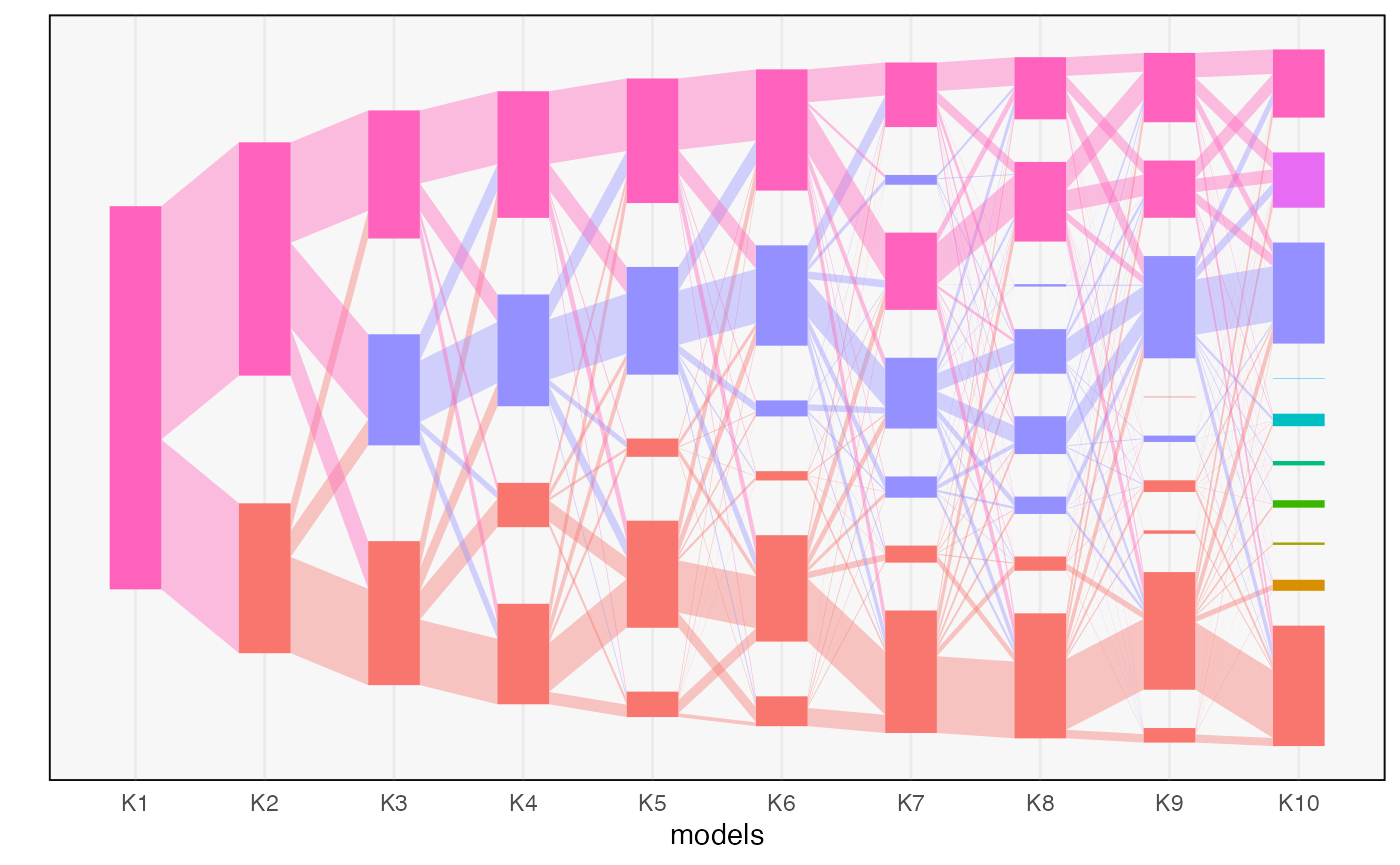

plot_beta(alignment, c(2, 4))

We can plot measures of topic quality across \(m\). The introduction of a low quality topic at \(K = 4\) is consistent with the fact that there are only 3 true topics in this data.

ggplot(topics(alignment), aes(m, coherence)) +
  geom_point(alpha = 0.5)


ggplot(topics(alignment), aes(m, refinement)) +
  geom_point(alpha = 0.5)
#> Warning: Removed 10 rows containing missing values (`geom_point()`).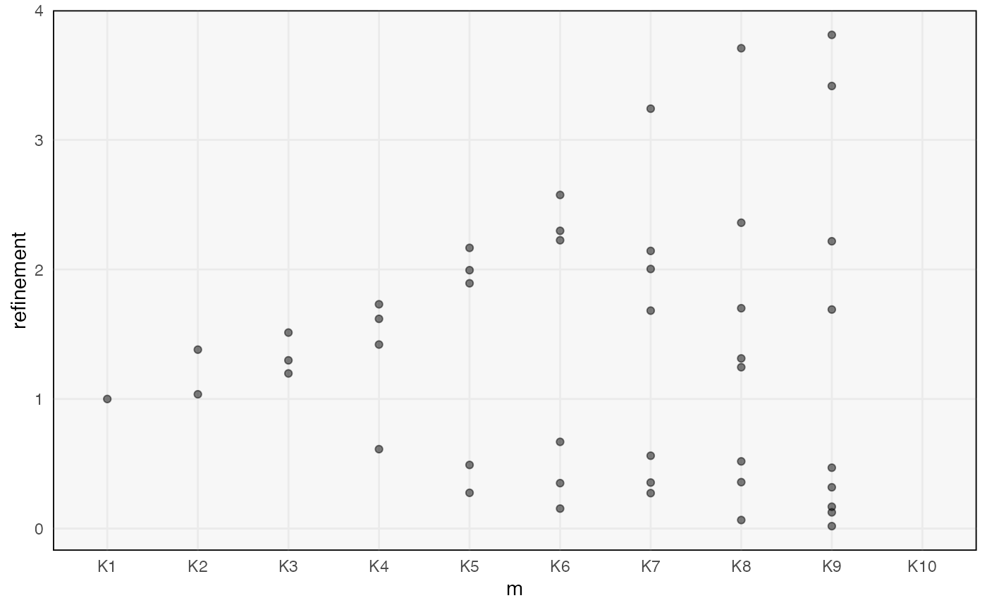

We can also compute the number of key topics associated with the alignment.

key_topics <- compute_number_of_paths(alignment) %>%
  mutate(id = id)

Finally, we save all the results (if wanted). The distinct IDs allow us to gather alignments from across many replicates, and these are what are shown in the simulation section of the manuscript.

id_vars <- params[c("out_dir", "method", "id", "N", "V", "K")]
scores <- topics(alignment) %>%
  mutate(id = id)

if (save) {
  dir.create(out_dir, recursive = TRUE)
  write_csv(key_topics, save_str("key_topics", id_vars))
  write_csv(scores, save_str("topics", id_vars))
  exper <- list(x, betas, gammas, alignment)
  save(exper, file = save_str("exper", id_vars, "rda"))
}

if (perplexity & save) {
  x_new <- simulate_lda(betas, gammas, lambda = lambdas$count)
  perplexities <- matrix(nrow = n_models - 1, ncol = 2, dimnames = list(NULL, c("train", "test")))
  for (k in seq(2, n_models)) {
    load(str_c("fits/lda_K", k, ".Rdata"))
    perplexities[k - 1, 1] <- topicmodels::perplexity(tm, x)
    perplexities[k - 1, 2] <- topicmodels::perplexity(tm, x_new)
  }

  cbind(K = seq(2, n_models), perplexities) %>%
    as_tibble() %>%
    write_csv(save_str("perplexity", id_vars))
}