Introduction to Alignment
basic-alignment.RmdThis vignette describes the main functions of the alto
package on a simple simulated dataset. We will introduce,
-
run_lda_modelsfor fitting a sequence of LDA models to a fixed dataset -
align_topicsfor aligning topics across a set of fitted models -
plotandplot_betafor displaying the results
First, we load some packages that are used in this vignette.
Next, we simulate a dataset (50 samples with 20 dimensions each)
samples and run a sequence of LDA models to it. The data,
x, are all independent multinomials and there is no
low-rank structure for any models to learn. Nonetheless, it is
sufficient for illustrating the package.
The arguments to run_lda_models are the matrix
x and a list of lists, lda_params, which
specifies how hyperparameters are to be varied across the sequence of
models. The \(i^{th}\) element of the
list contains hyperparameters that will be used in the \(i^{th}\) model fit. Any hyperparmeters that
are accepted by topicmodels::LDA can be passed into these
internal lists. We use map to construct a list whose \(i^{th}\) element specifies that the \(i^{th}\) LDA model should fit \(k = i\) topics.
x <- rmultinom(20, 500, rep(0.1, 50))
colnames(x) <- seq_len(ncol(x))
lda_params <- setNames(map(1:10, ~ list(k = .)), 1:10)
lda_models <- run_lda_models(x, lda_params)
#> Using default value 'VEM' for 'method' LDA parameter.
#> Using default value 'VEM' for 'method' LDA parameter.
#> Using default value 'VEM' for 'method' LDA parameter.
#> Using default value 'VEM' for 'method' LDA parameter.
#> Using default value 'VEM' for 'method' LDA parameter.
#> Using default value 'VEM' for 'method' LDA parameter.
#> Using default value 'VEM' for 'method' LDA parameter.
#> Using default value 'VEM' for 'method' LDA parameter.
#> Using default value 'VEM' for 'method' LDA parameter.
#> Using default value 'VEM' for 'method' LDA parameter.
The output of this function is a list of two element lists. The first element are the mixed-membership estimates \(\gamma\). This is an \(N \times K\) matrix specifying the membership of each sample across the \(K\) topics. THe second element are the estimated topic log-probabilities, \(\log\beta\). This is a \(K \times D\) matrix whose rows give the log probabilities for each dimension within that topic.
Given this output, we can compute a tpoic alignment. This is done by
the align_topics function. By default, the
product method is used to compute weights (below, we show
how to use the transport or more custom methods).
This function returns an object of class alignment. Its
print method shows the topic weights between pairs of topics across
models. The first two columns give the index \(m\) of the models from the input. The next
two columns give the index \(k\) of
topics within those models. For example, the first row gives the
alignment between the first topics estimated in the \(K = 1\) and \(K =
2\) models. Since there is no low-rank structure in this model,
all outgoing weights from a given topic are equal.
result <- align_topics(lda_models)
result
#> # An alignment: 10 models, 55 topics:
#> # A tibble: 6 × 8
#>   m     m_next     k k_next weight document_mass bw_weight fw_weight
#>   <fct> <fct>  <int>  <int>  <dbl>         <dbl>     <dbl>     <dbl>
#> 1 1     2          1      1  0.500          25.0         1     0.500
#> 2 1     2          1      2  0.500          25.0         1     0.500
#> 3 1     3          1      1  0.333          16.7         1     0.333
#> 4 1     3          1      2  0.333          16.7         1     0.333
#> 5 1     3          1      3  0.333          16.7         1     0.333
#> 6 1     4          1      1  0.250          12.5         1     0.250
#> # ... with 1314 more rows
We can access the full weights (not just the first few rows), by
using the weights method.
weights(result)
#> # A tibble: 1,320 × 8
#>    m     m_next     k k_next weight document_mass bw_weight fw_weight
#>    <fct> <fct>  <int>  <int>  <dbl>         <dbl>     <dbl>     <dbl>
#>  1 1     2          1      1  0.500          25.0         1     0.500
#>  2 1     2          1      2  0.500          25.0         1     0.500
#>  3 1     3          1      1  0.333          16.7         1     0.333
#>  4 1     3          1      2  0.333          16.7         1     0.333
#>  5 1     3          1      3  0.333          16.7         1     0.333
#>  6 1     4          1      1  0.250          12.5         1     0.250
#>  7 1     4          1      2  0.250          12.5         1     0.250
#>  8 1     4          1      3  0.250          12.5         1     0.250
#>  9 1     4          1      4  0.250          12.5         1     0.250
#> 10 1     5          1      1  0.200          10.0         1     0.200
#> # ℹ 1,310 more rows
The align_topics function also computes a few per-topic
measures. These can be accessed using topics. For example,
mass describes the total mass \(\sum_{i =
1}^{n}\gamma_{ik}^{m}\) for topic \(k\) in model \(m\). The prop column
normalizes the mass column according to the total mass
within that model. branch specifies which overall branch
each topic belongs to (this corresponds to colors in the flow diagrams
below). Coherence and refinement are complementary measures of topic
quality. For details on their properties, please refer to the manuscript
accompanying this package.
topics(result)
#> # A tibble: 55 × 8
#>    m         k k_label  mass  prop path  coherence refinement
#>    <fct> <int> <fct>   <dbl> <dbl> <fct>     <dbl>      <dbl>
#>  1 1         1 1        50   1     2         0.293       1
#>  2 2         1 1        25.0 0.500 2         0.293       1.00
#>  3 2         2 2        25.0 0.500 7         0.245       1.00
#>  4 3         1 1        16.7 0.333 2         0.237       1.00
#>  5 3         2 3        16.7 0.333 2         0.237       1.00
#>  6 3         3 2        16.7 0.333 7         0.245       1.00
#>  7 4         1 1        12.5 0.250 2         0.219       1.00
#>  8 4         2 3        12.5 0.250 2         0.219       1.00
#>  9 4         3 4        12.5 0.250 9         0.247       1.00
#> 10 4         4 2        12.5 0.250 7         0.235       1.00
#> # ℹ 45 more rows
An alternative measure is the key_topics measure. This
looks at how many topics have similar descendents across resolution
levels, and it can be accessed using the
compute_number_of_key_topics function,
compute_number_of_paths(result, plot=TRUE)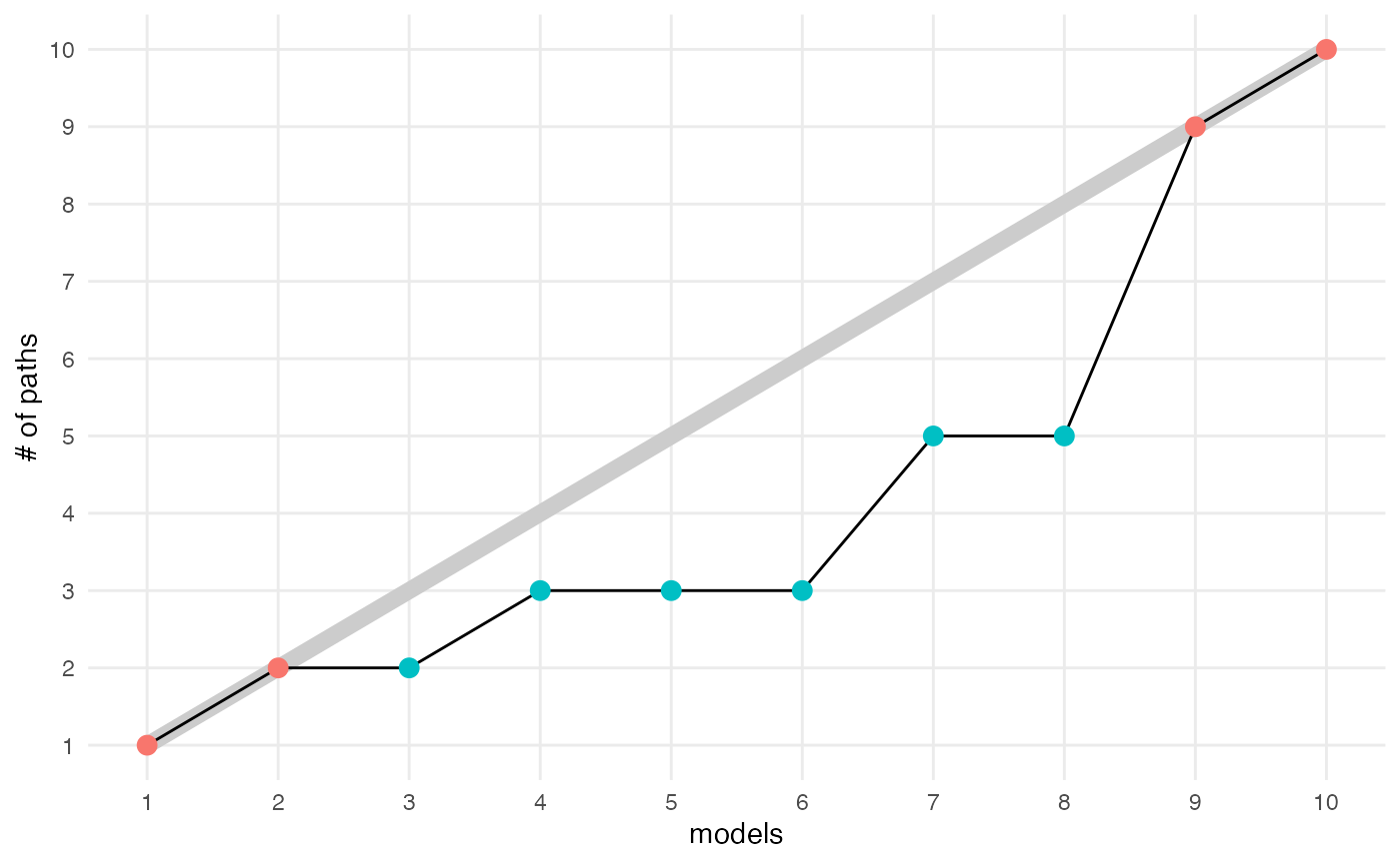
#> # A tibble: 10 × 3
#>    m     n_paths n_topics
#>    <fct>   <int>    <int>
#>  1 1           1        1
#>  2 2           2        2
#>  3 3           2        3
#>  4 4           3        4
#>  5 5           3        5
#>  6 6           3        6
#>  7 7           5        7
#>  8 8           5        8
#>  9 9           9        9
#> 10 10         10       10
Visualizations
The information in the weights and topics
functions can be displayed visually using the alignment
class’ plot method. Each column in the flow diagram
corresponds to one model, and each rectangle gives a topic. The height
of each rectangle gives the topic mass defined above. The size of the
edges between rectangles corresponds to the weight of that edge in the
alignment. In this multinomial dataset, the perfect “fanning” structure
suggests that there is no topic structure – there are no emergent
branches. This makes sense, since there is no low-rank structure when
simulating a 50-dimensional multinomial.
plot(result)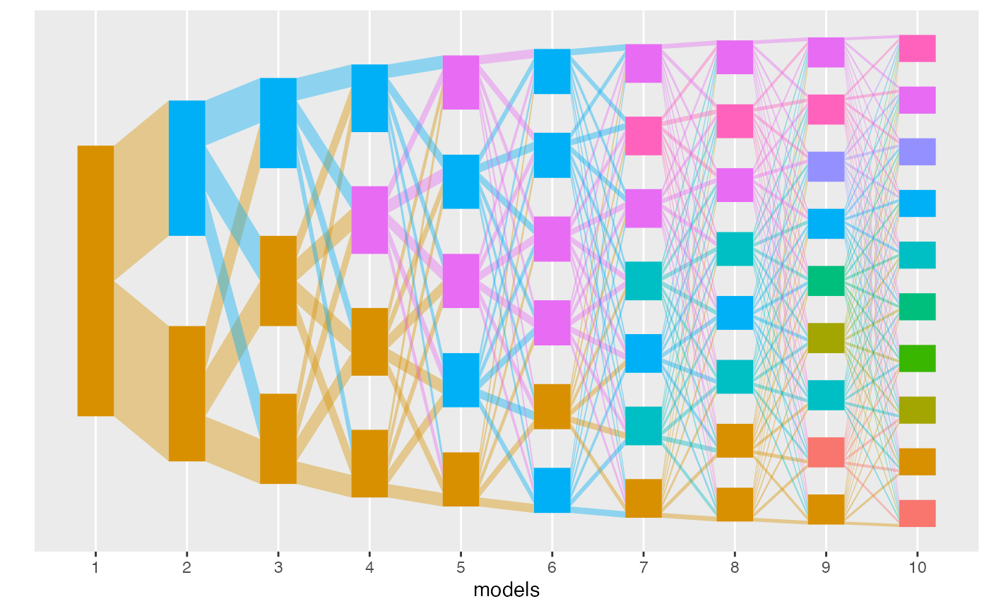
By default, plot shades each topic and edge in according
to its branch membership. We could alternatively color by refinement,
robustness, or topic ID.
plot(result, color_by = "refinement")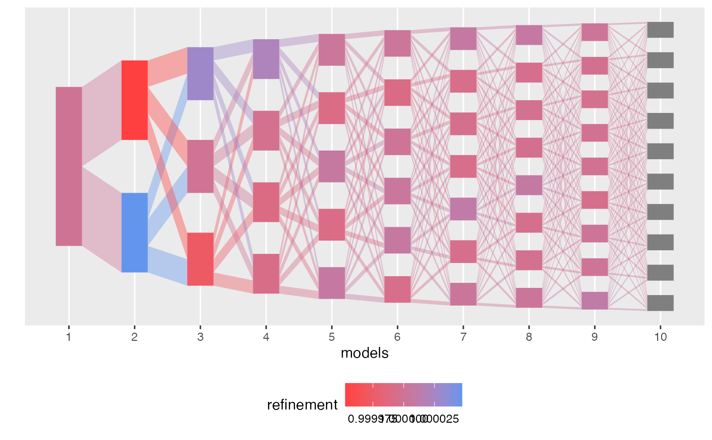
plot(result, color_by = "coherence")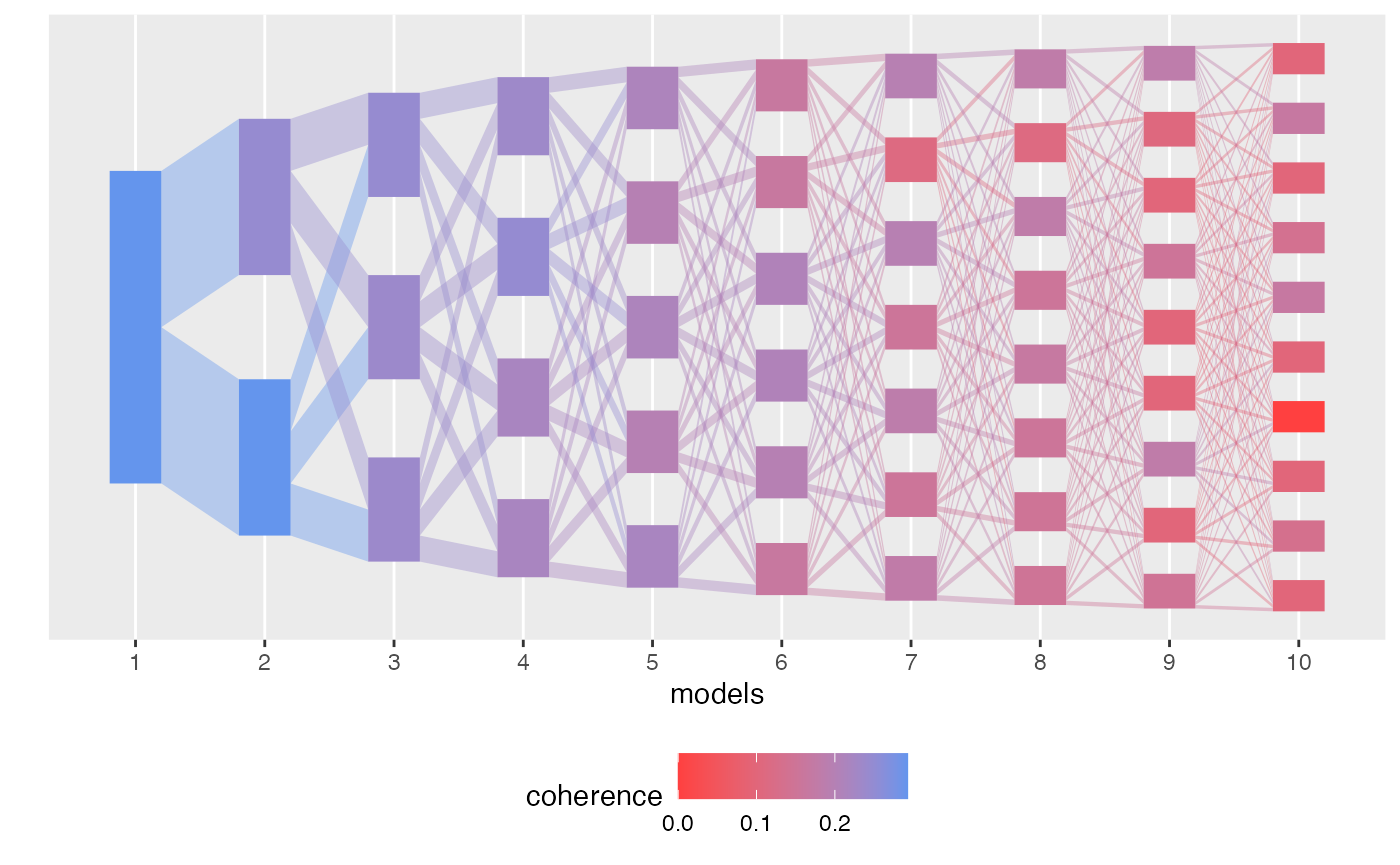
plot(result, color_by = "topic")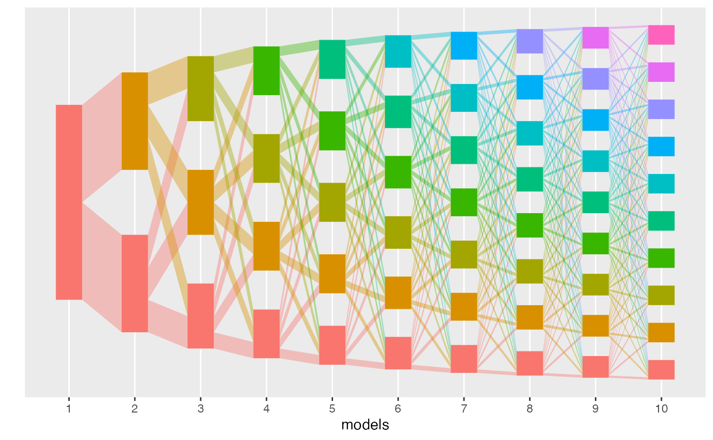
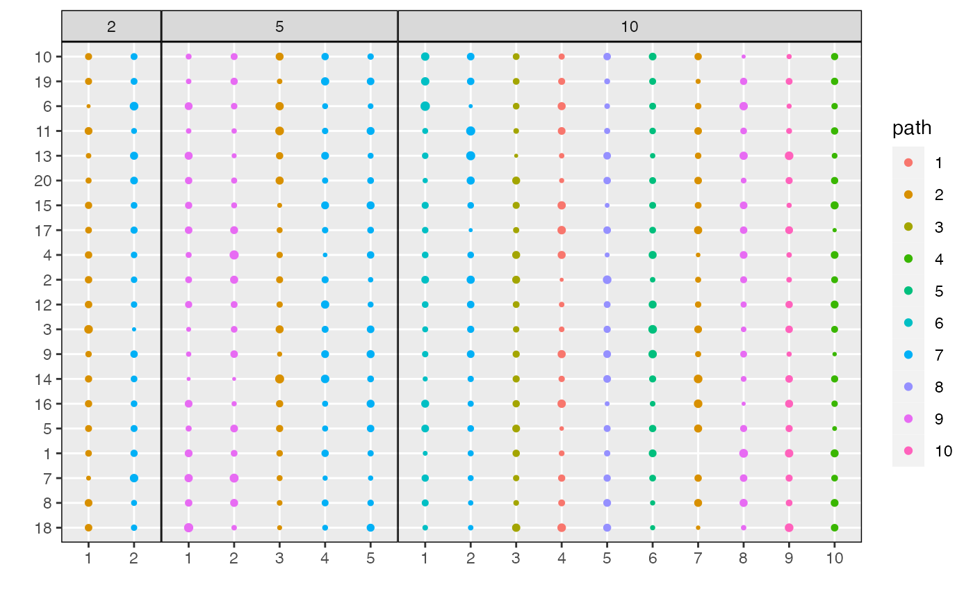
To understand the content of the topics, we can use
plot_beta. This shows the probabilities \(\beta_{kd}^{m}\) across topics and models.
Dimensions are sorted from those with the highest distinctiveness across
topics to those with the lowest. By default, all dimensions \(d\) with at least one \(\beta_{kd}^{m} >
0.001\) will be displayed. This can be adjusted using the
min_beta parameter. For clarity, circles with \(\beta_{kd}^{m} < \text{min_beta}\) are
not shown.
plot_beta(result)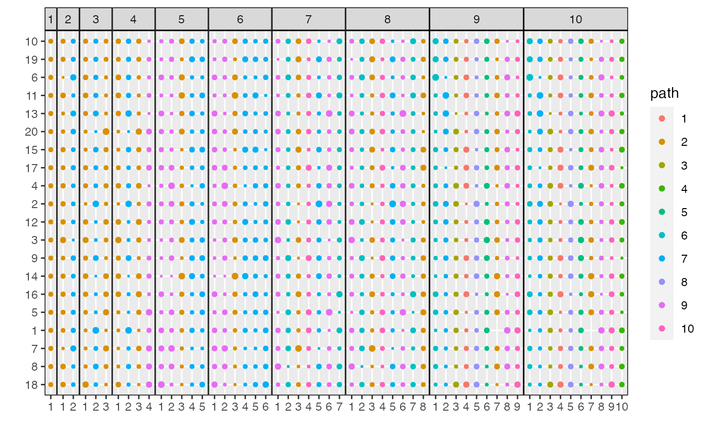
plot_beta(result, threshold = 0.05)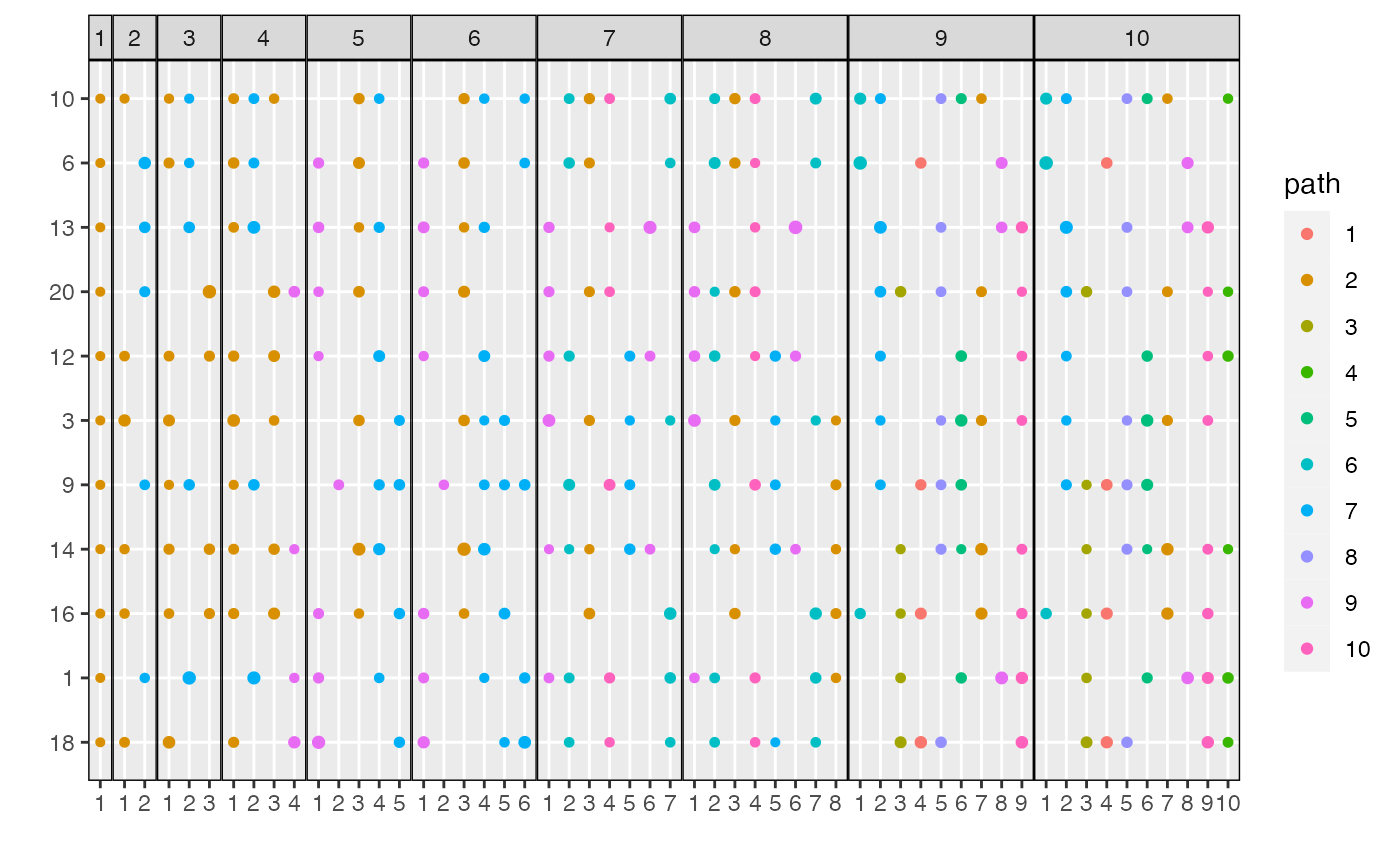
Alternatively, we can filter the number of dimensions shown using the
n_features parameter.
plot_beta(result, n_features = 5)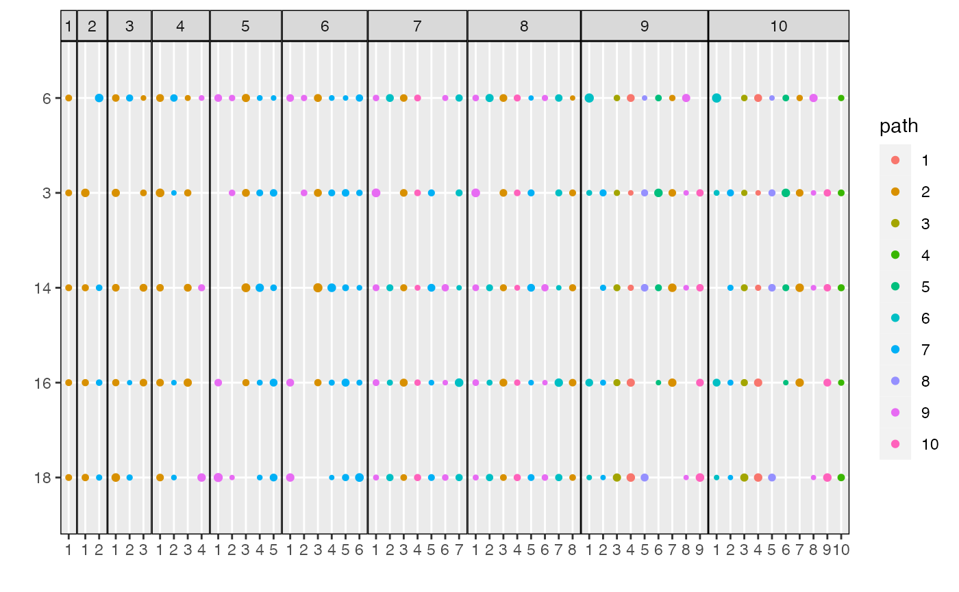
Finally, we can visualize topics associated with subsets of models,
either by specifying the name of that model in the
lda_models list or giving the model index.

plot_beta(result, "last")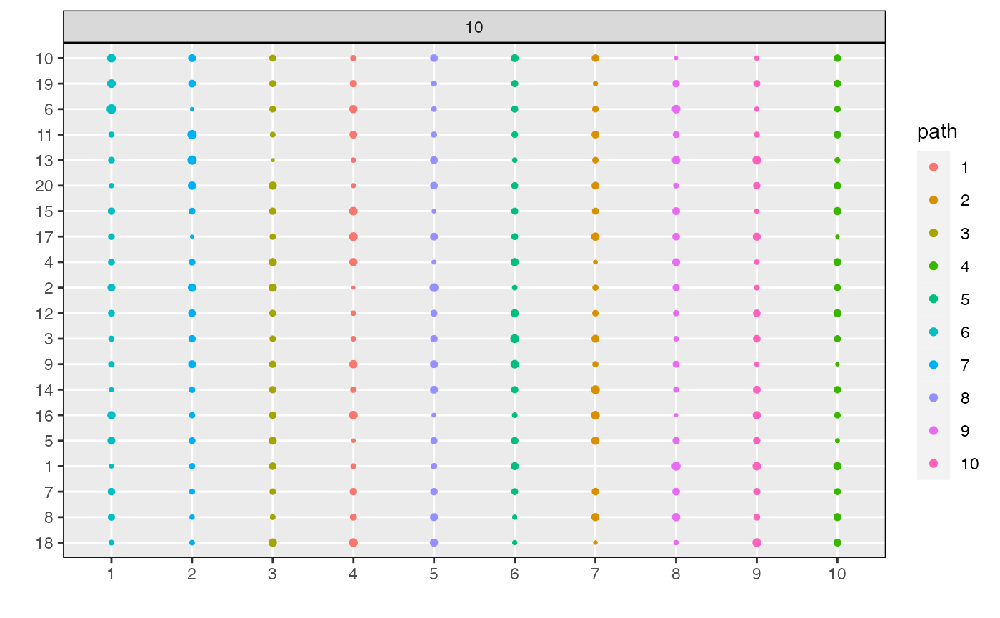
Alternative Alignments
We can compute an alignment using the transport approach using the
method argument.
result <- align_topics(lda_models, method = "transport")
plot(result)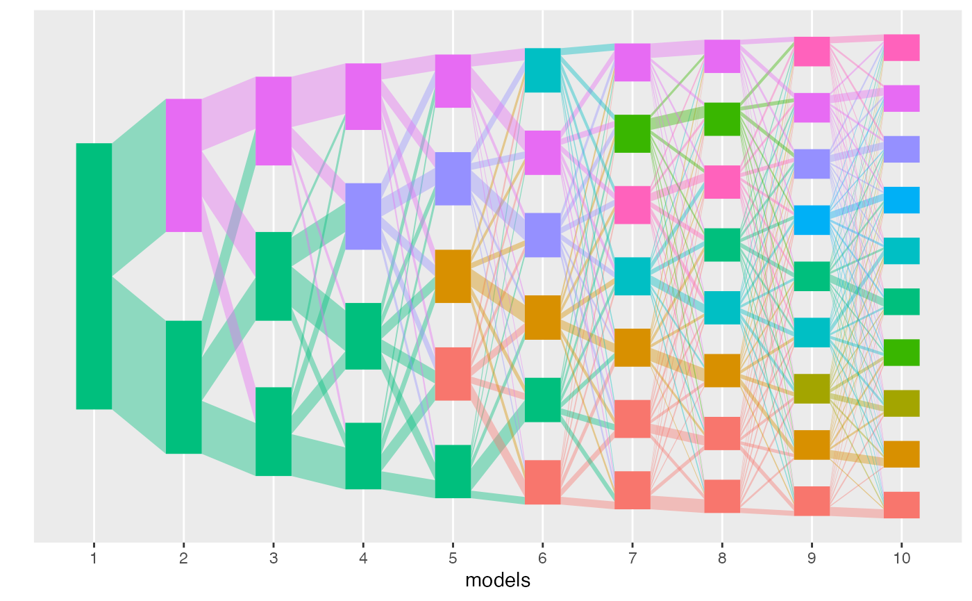
align_topics computes an alignment sequentially across
the input gamma and beta lists. In principle,
an alignment can be computed between arbitrary pairs of topics. This
functionality is supported by the align_graph function. For
example, we can fit an alignment between all pairs of topics, across all
models.
edges <- alto:::setup_edges("all", names(lda_models))
gamma <- map(lda_models, ~ .$gamma)
beta <- map(lda_models, ~ 2 ^ .$beta)
align_graph(edges, gamma, beta, transport_weights)
#> # A tibble: 1,320 × 8
#>    m     m_next     k k_next weight document_mass bw_weight fw_weight
#>    <fct> <fct>  <int>  <int>  <dbl>         <dbl>     <dbl>     <dbl>
#>  1 1     2          1      1  0.500          25.0         1     0.500
#>  2 1     2          1      2  0.500          25.0         1     0.500
#>  3 1     3          1      1  0.333          16.7         1     0.333
#>  4 1     3          1      2  0.333          16.7         1     0.333
#>  5 1     3          1      3  0.333          16.7         1     0.333
#>  6 1     4          1      1  0.250          12.5         1     0.250
#>  7 1     4          1      2  0.250          12.5         1     0.250
#>  8 1     4          1      3  0.250          12.5         1     0.250
#>  9 1     4          1      4  0.250          12.5         1     0.250
#> 10 1     5          1      1  0.200          10.0         1     0.200
#> # ℹ 1,310 more rows
Finally, arbitrary weight methods can be passed to
align_graph. The only requirement is that, given pairs of
matrices of mixed-memberships and log-topics between two models, the
function must return a data.frame of weights between all pairs of
topics. The transport_weights function above is an
example,
transport_weights(gamma[1:2], beta[1:2])
#> # A tibble: 2 × 3
#>   k     k_next weight
#>   <chr> <chr>   <dbl>
#> 1 1     1        25.0
#> 2 1     2        25.0
Here is a dummy example that always returns a weight of 0 between all pairs of topics.
dummy_weights <- function(gamma, beta) {
  zeros <- matrix(0, ncol(gamma[[1]]),nrow(gamma[[2]]))
  alto:::.lengthen_weights(data.frame(zeros))
}

align_graph(edges, gamma, beta, weight_fun = dummy_weights)
#> # A tibble: 8,250 × 8
#>    m     m_next     k k_next weight document_mass bw_weight fw_weight
#>    <fct> <fct>  <int>  <int>  <dbl>         <dbl>     <dbl>     <dbl>
#>  1 1     2          1      1      0             0       NaN       NaN
#>  2 1     2          1      2      0             0       NaN       NaN
#>  3 1     2          1      3      0             0       NaN       NaN
#>  4 1     2          1      4      0             0       NaN       NaN
#>  5 1     2          1      5      0             0       NaN       NaN
#>  6 1     2          1      6      0             0       NaN       NaN
#>  7 1     2          1      7      0             0       NaN       NaN
#>  8 1     2          1      8      0             0       NaN       NaN
#>  9 1     2          1      9      0             0       NaN       NaN
#> 10 1     2          1     10      0             0       NaN       NaN
#> # ℹ 8,240 more rows