Research
Identifying reproductive events in time series of self-reported fertility body signs
The first step towards investigating the effects of the menstrual cycle and, more generally, reproductive status (contraception, pregnancies, pregnancy losses) on other aspects of health is to have tools that identify reproductive events. While lab tests measuring a series of hormones or ultra-sound imagery are gold standards for detecting ovulation or pregnancy stages, they are expensive and virtually impossible to deploy on large longitudinal cohorts. At the same time, menstrual cycle and fertility tracking on smartphone apps has become ubiquitous. There are now millions of women around the globe using these apps, sometimes over the course of several years. I thus wanted to examine whether they could offer a more practical alternative to expensive laboratory methods for identifying reproductive status.
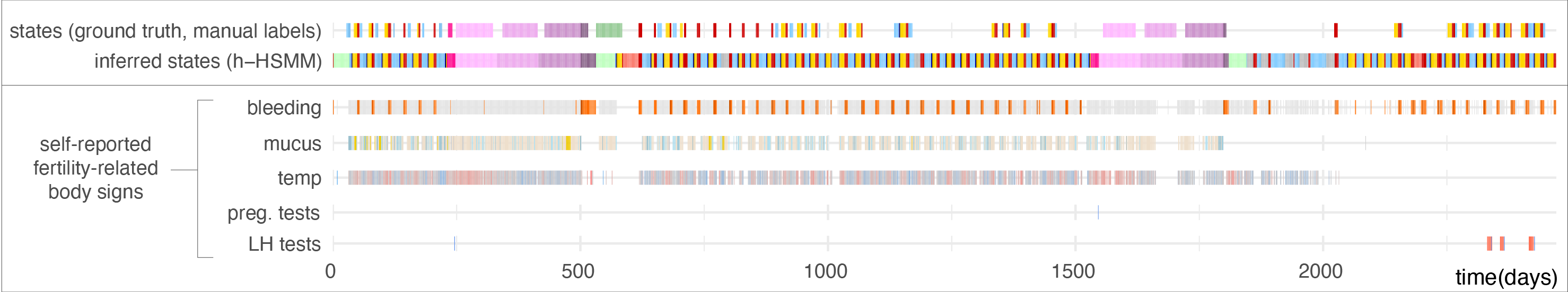
A first study evaluates whether self-reported fertility body signs during ovulatory cycles matched the expected patterns reported from medical studies. Following the positive results of this first study, my next pursuit was to detect reproductive events such as ovulation, early pregnancy losses, births, and breastfeeding within the full time series reported by app users. I used hidden semi-Markov models to describe reproductive events as a sequence of hidden states (see study, software (HiddenSemiMarkov R package), and figure below). We showed that hidden semi-Markov models performed better than hidden Markov models, which demonstrated the added value of a Bayesian method that incorporates biomedical knowledge about state duration into the model. We also showed that the hierarchical approach used to account for changes in tracking behavior improved the detection of long-duration events such as pregnancies or breastfeeding.
These models are now included in another R package which I have developed which implements the C-PASS procedure for the diagnosis of PMDD (premenstrual dysphoric disorder). C-PASS normally relies on manual identification of menstrual cycle phases, whereas the cpass R package I developed uses these models to automate this identification process.
Sub-communities of the vaginal microbiome
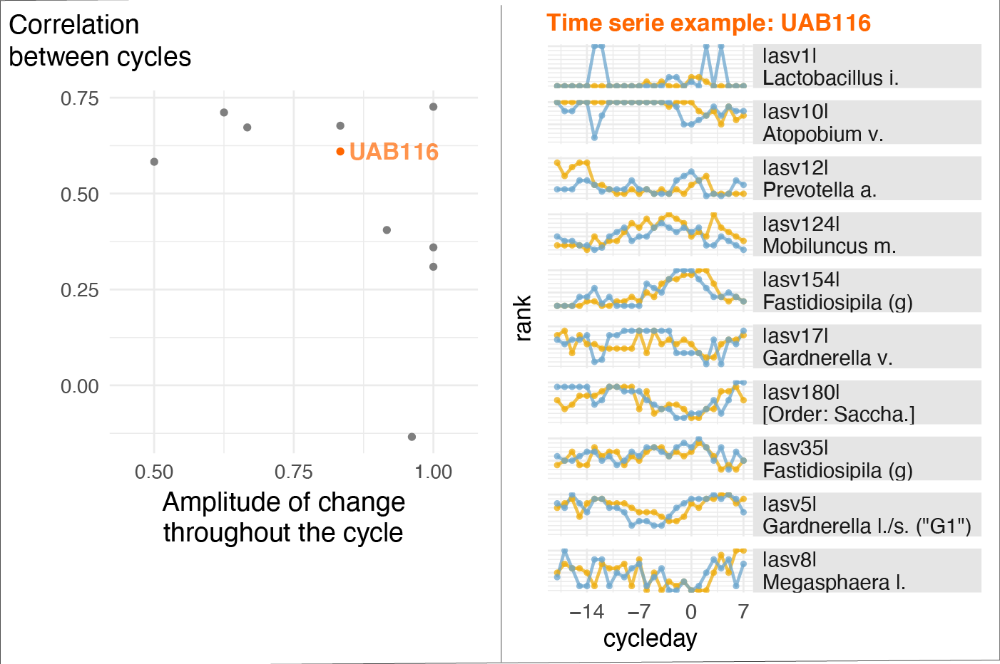
This project is a primary example of a study where accounting for menstrual cycle timing played a key role in understanding another physiological phenomenon: in this case, changes in the vaginal microbiota (VM) composition. The study is part of the efforts of the Vaginal Microbiome Research Consortium (VMRC), which is funded by the Gates Foundation and directed by Prof. Ravel (University of Maryland) and Prof. Relman (Stanford University). Using longitudinal data from menstruating individuals over two cycles, we found that within-subject variations in VM compositions were highly correlated from one cycle to the next (see figure below). Moreover, we found that the concentrations of many metabolites and cytokines peaked at specific phases of the menstrual cycle. This may suggest that an intervention aimed at shifting the VM composition (e.g., for health reasons) could be optimally timed within the menstrual cycle. Non-optimal VM composition has been shown to be associated with a series of negative health outcomes such as increased risk of preterm birth, contracting a sexually transmitted infection including HIV, or painful menstruation.
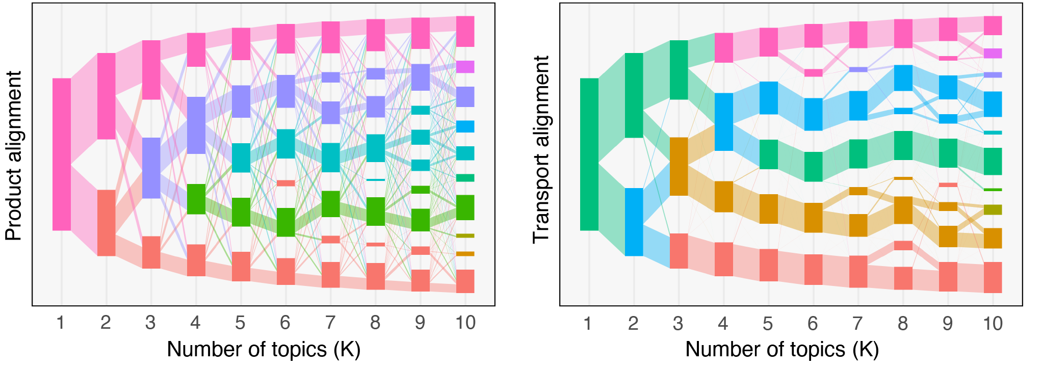
Beyond characterizing the effects of the menstrual cycle on the VM composition, my contribution also included using mixed membership models (topic models) to characterize the structure of these non-optimal states. In particular, we identified several sub-communities (i.e., groups of co-existing or functionally equivalent bacterial strains) in samples from both pregnant and non-pregnant subjects. This agreement across cohorts suggests that these sub-communities are biologically meaningful, rather than artifacts of our model. My current work within the VMRC focuses on deploying and developing data integration methods to better understand the interactions between the various micro-environment elements of the multi-omics VMRC dataset. Such methods include topic alignment (see figure below) across modalities, an extension of the framework proposed earlier this year by Dr. Fukuyama (Indiana University), Dr. Sankaran (UW Madison), and myself.
Seasonal fertility
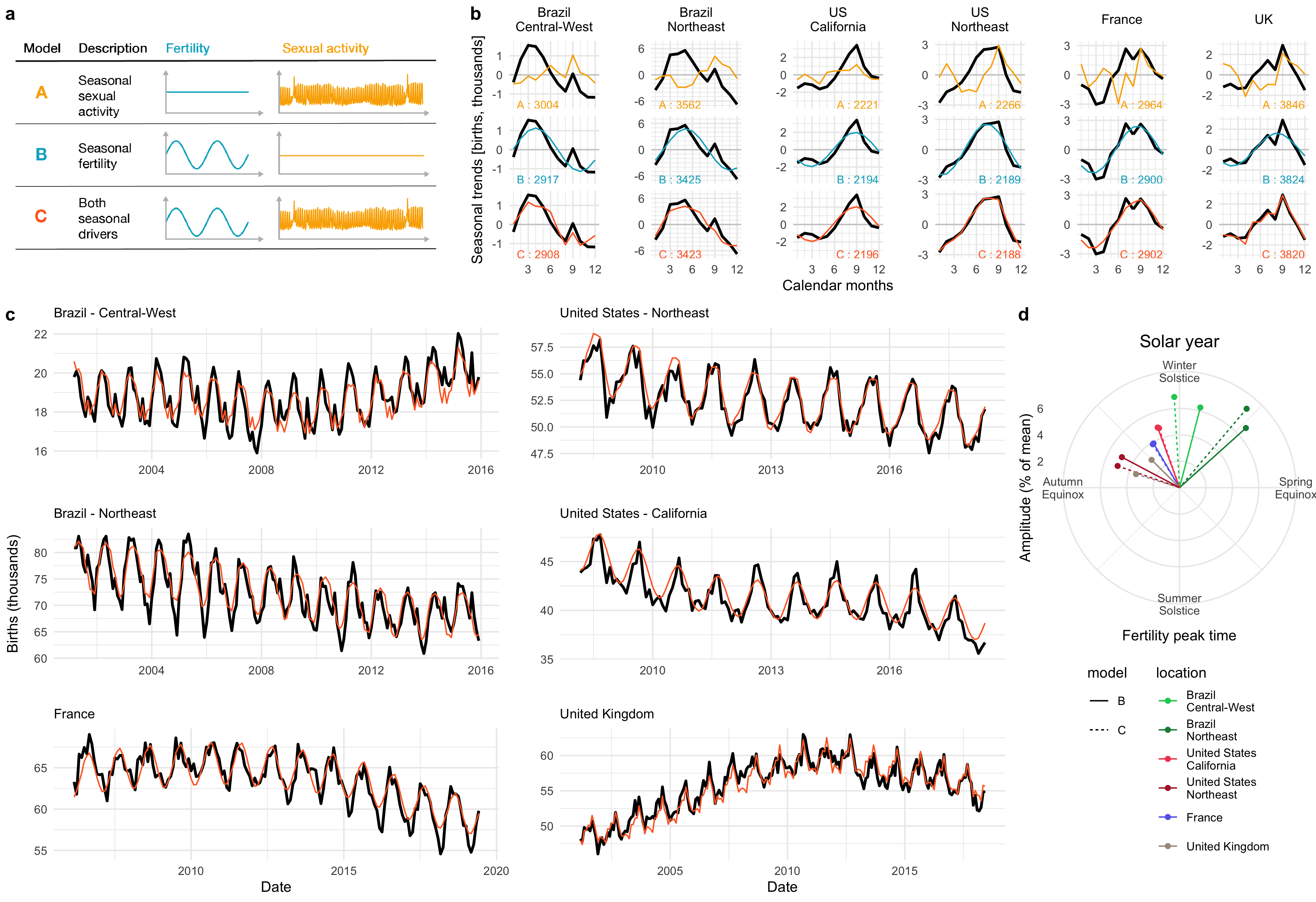
Although humans can reproduce all year round, historical records show seasonal oscillations of birth rates. Moreover, seasonal birth rate patterns vary based on location. To investigate whether these seasonal changes in birth rates resulted from changes in sexual activity or fertility, we analyzed self-reported sexual activity data from over half a million users of a menstrual cycle app, Clue, from six locations across both hemispheres. Fitting a statistical model of birth rates from sexual activity and fertility rates to our data indicated that while an increase in sexual activity during local holidays contributed to local peaks in the birth curves, the seasonal changes in births were more likely explained by seasonal changes in fertility. This project was done in collaboration with Prof. Martinez, previously at Columbia University, now at Emory University, and as part of an on-going collaboration with BioWink GmHB, owner of the Clue app, whose data we used for this study.
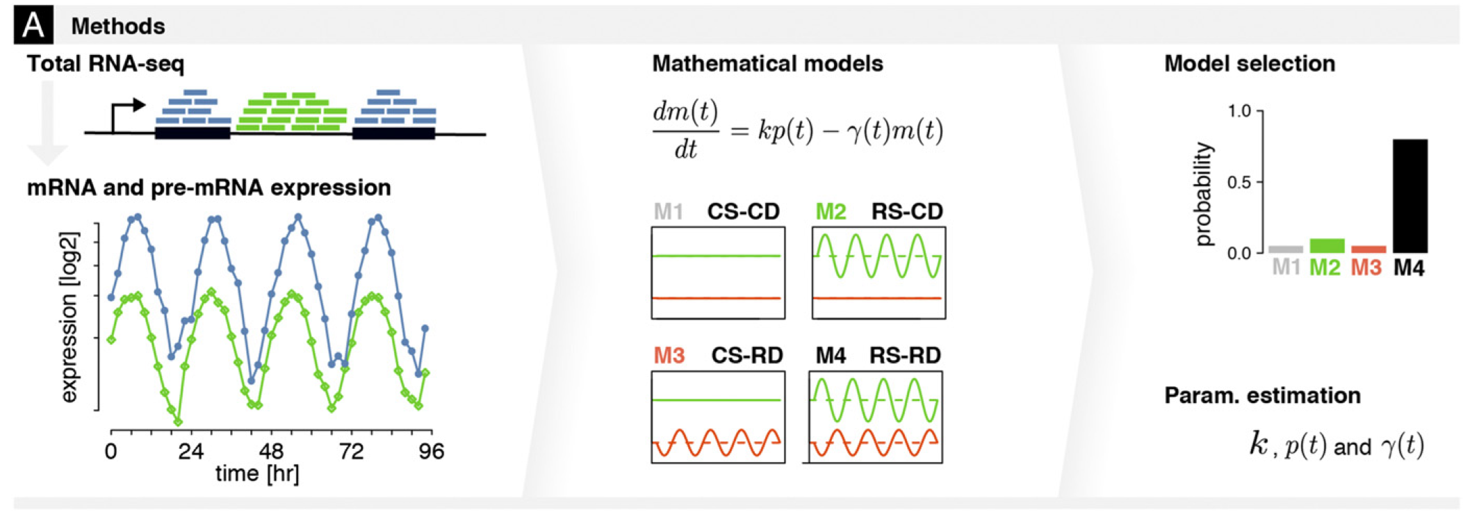
Transcriptional and posttranscriptional regulation of the mammalian circadian clock
During my PhD in computational biology at EPFL, I authored a series of studies that each focused on a specific step of the circadian regulation of gene expression. Altogether our work showed that rhythmic gene expression (i.e., oscillations in gene expression with a 24-hour period) may result from rhythmic binding of transcription factors to gene promoters, rhythmic activity of the transcriptional machinery, rhythmic degradation of gene transcripts, or from rhythmic translational activity due to differential abundance of ribosomal RNA. Each of these studies relied on statistical analyses of periodic signals identified in multi-omics datasets. My work on identifying which transcripts were rhythmically degraded required the establishment of models describing variations in transcript abundance. While transcript degradation rates are not directly measurable, our models enabled us to infer the degradation rates from transcript production and accumulation rates, which are measurable. These models also allowed us to estimate the probability for a transcript to undergo rhythmic (vs. constant) degradation.